Making genetic maps is a basic skill for genetic studies. F2 and recombinant inbred lines (RILs) are the most popular populations. RILs are usually selfed for 5 or more generations, so treated as homozygous lines and heterozygous markers were set to missing data. Mapmaker is the most classic map-making software when the number of markers is small (maximum a few hundred). MapMaker is very old and not easy to use. I found R/qtl and onemap uses the same ideas as Mapmaker and both have the “ripple” function, locally finding the best order. However, they cannot handle today’s high-density markers, usually more than 1000. I found the best free software is ASMap, which is an R package based on MSTmap. It has a very good tutorial with detailed instructions on making a good genetic map. Here is a simple summary based on my experience and the ASMap vignette.
Call SNPs using Genome Studio 2
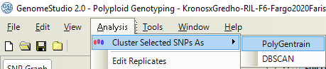
If you are using wheat 9K or 90K SNP arrays, I suggest getting the raw Genome Studio file from the genotyping lab. Then you can call SNPs with PolyGentrain method (Menu -> Analysis -> Cluster Selected SNPs As -> PolyGentrain).
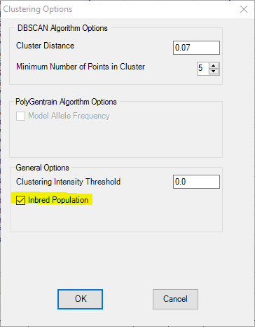
The default call will call 3 clusters: AA, AB, and BB. So if yours are inbred lines (only have AA and BB), please go to “Menu -> Tools -> Clustering Options” to check the “Inbred Population” checkbox.
Another trick to easily check only a subset of markers is to use filters.
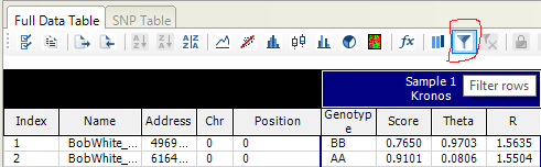
After clicking the filter icon, a window will pop up. Make a simple filter, then save it to a file, say tmp. When you click “Save” another time, then it will warn you whether you want to overwrite the old file. Here you can find the location of the filter file and you can open it with a text editor. You can edit this file and load it from Genome Studio to get the lines you want easily and fast.
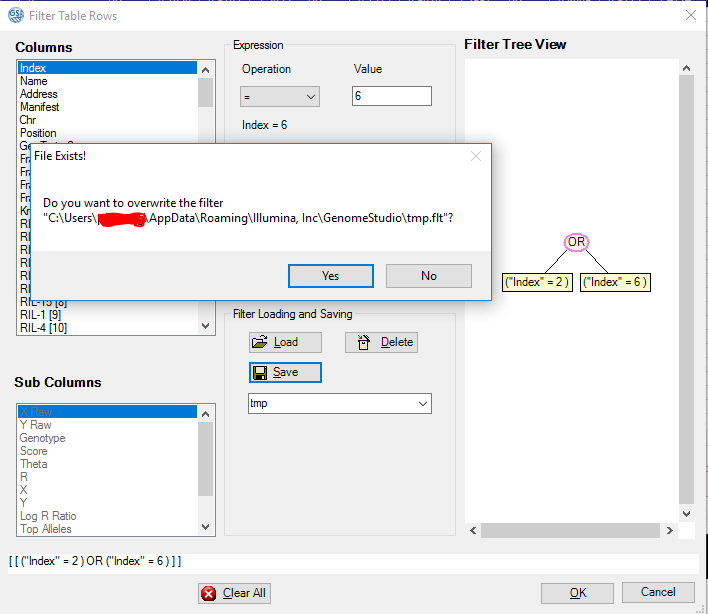
This way you can quickly check hundreds of markers that might have clustering problems during map construction.
Pre-construction
Now we often have thousands of markers, it is not a big deal to filter out those with low quality.
- Missing data. I only keep markers with <10% of missing data. Lines with too many missing data were also removed (I do not have a number here, 20% is a good start, usually I will plot to find the outliers).
- Check lines with high similarity (>95%) and only keep 1 of them.
- Check for co-locating markers. Only keep 1 marker of each group to reduce the calculating cost.
- Check markers for excessive segregation distortion. Usually, we use the Chi-square test or Bonferroni corrected Chi-square test (corrected pvalue = raw pvalue / number of markers). I use the Bonferroni corrected chi-square test P = 0.05 as the threshold after removing co-located markers. It is normal to have some regions with segregation distortion.
ASMap has all the tools to help you clean your data before map construction.
During construction
You can make genetic maps step by step based on the ASMap vignette. I found F2 and RILs have a little difference, so I made 2 exmaple R scripts and real-world examples:
Depending on the diversity of your mapping parents and marker distribution, the short arm and long arm of some chromosomes might not be able to be connected by markers: no close markers in between. We can either keep them as separated arms or push them together as one complete chromosome but with big gaps between arms.
We need to try different p values in function “mstmap” to split markers into groups that only belong to unique chromosomes. If the p value is too big, say 1e-6, markers from homeolog chromosomes such as 1A and 1B might still cluster together. For wheat RILs, 1e-10 is a good start. After splitting them into clusters, then we can check their physical location, and then merge some groups if they come from the same chromosome.
Post construction with ASMap
Maps from ASMap have good marker orders. Due to genotyping errors, there are always several orders that can make the map the shortest. ASMap might use a fixed seed, so its output is always the same. We can use tspOrder2 to check other possible marker orders and select the one that is the most consistent with the physical map.
I also suggest to the thin the markers before QTL analysis. If you have 4000 markers, the QTL mapping will be very slow without much resolution improvement. You can use the “dropSimilarMarkers” function in the script junli-genetic-map-functions.R to drop too close markers (default recombination frequency 0.01).
If you want to draw genetic maps from your final result, please try RgeneticMap.
